1. Purpose
- Experiment with computer vision and autonomous navigation
- Continue and improve Robot Navigation using Stereo Vision using home-made stereo camera module
2. Components
- TeensyCam - stereo camera module based on MT9V034 sensors
- LattePanda single board computer
- Teensy 3.2 microcontroller
- DFRobot Cherokey 4WD Mobile Platform
- NiMH 2500mAh AA batteries (7 pcs)
- Graupner 6425 NiMH charger
- BNO055 - Absolute Orientation Sensor
3. Results
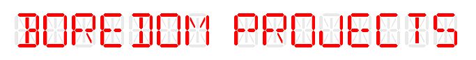
I'd like to introduce a robot called Heisenberg! He doesn't do much, other than driving around. He is, however, aware of his own health and the environment around him. He speaks and understands speech. He knows where he is and where he wants to go, well, most of the time. He makes mistakes and stumbles upon things, but that's what makes him human robot!
One more video where Heisenberg complains about low battery and tries to go back to base to recharge. Of course, at this point, he cannot recharge without human help yet, but I'm working on it...
More videos are here.
4. Progress Report
4.1. Intro
My first attempt to make a self-navigation robot using stereo vision was not exactly successfull. I thought the concept should be definitely doable, unfortunately, my problem was unsynchronized stereo camera (Minoru) that I was using back then. So, this time, I decided to overcome that limitation by building my own stereo camera module.
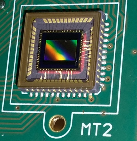
I discovered a suitable imaging sensor - MT9V034, which is a large, very sensitive imaging array with global shutter and hardware synchronization capability!
This project builds upon the Mobile Robotic Platform, which I created specifically for the purpose of experimentation with autonomous navigation. This platform was modified somewhat to fix various hardware issues. It has also been equipped with a custom-made stereo camera as a primary sensor.
4.2. Hardware
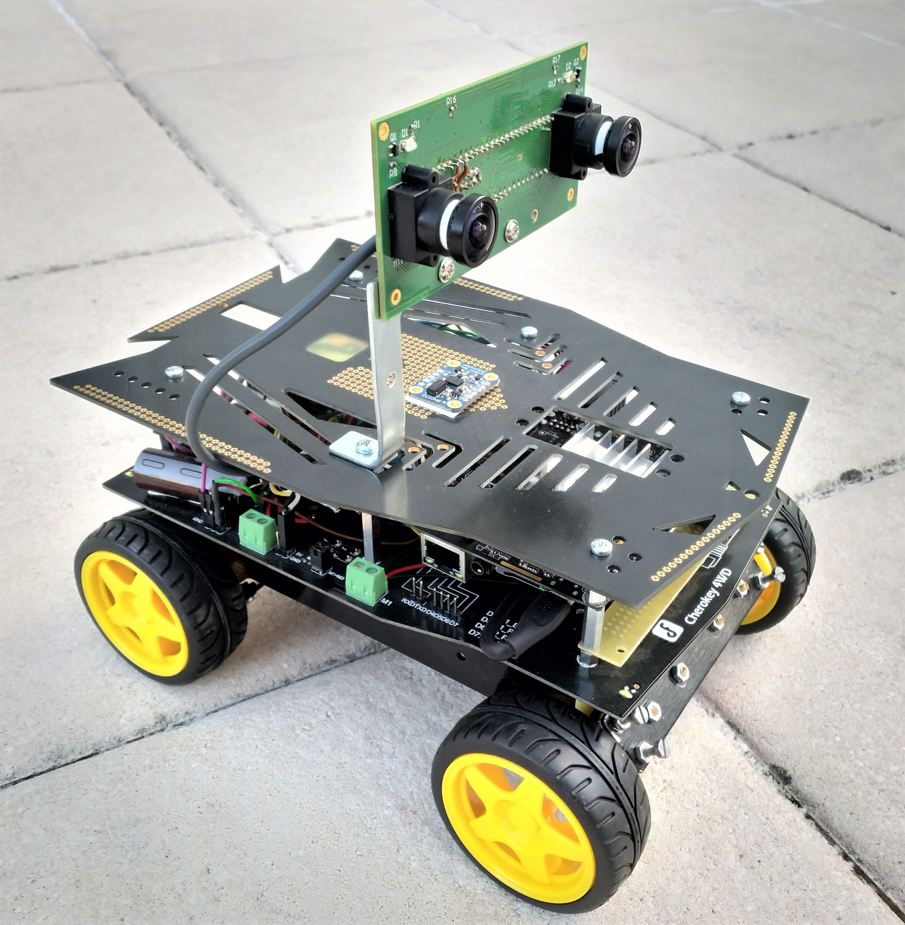
4.2.1. Camera
Doing away with Minoru webcam was not easy because it was just so damn cute! However, who can resist building a stereo camera module from scratch! 
First, some specs:
- Stereo baseline: 8 cm
- Resolution: 720 x 480 (vertical can be reduced to save bandwidth)
- Image format: raw, uncompressed, 10 bits per dot (monochrome)
- Interface: single USB 2.0 high speed port, CDC device profile
- Power: through USB, 150 mA
- Horizontal field of view: 105°
- Speed: 30 FPS max (configurable)
- Exposure: manual or automatic
- Global shutter, exposure synchronized by hardware
- Configurable number of lines to send to host
Design on GitHub here:
- Hardware: TeensyCam-HW
- Firmware: TeensyCam-SW
I discovered that MT9V034 monochrome sensor is actually quite popular and easy to use. A camera module based on it provides a two-fold advantage:
- Each of the two cameras uses global shutter, which means that all rows within a frame are exposed simultaneously. In a rolling shutter sensor, on the other hand, exposure and read out of each row happens in turn, as explained here. The resultant geometric distortions can break stereo disparity calculations when the robot is in motion or turning sharply. This becomes especially critical when driving during sub-optimum, indoor lighting conditions when exposure time is longer.

- Start of exposure is exactly synchronized by hardware between the two sensors. This is also obviously an important point for pretty much the same reasons as above.
The datasheet version D on the ON-Semi website actually does not provide register programming settings. Fortunately, an older version from Aptina can be easily found online, which does contain register descriptions. Using this info, as well as several programming references, such as this and this, I was able to successfully configure and use this module.
4.2.1.1. TeensyCam schematics

The four thick red lines on the schematic are due to post-design bug fixing. These connections are completed by soldering wires.
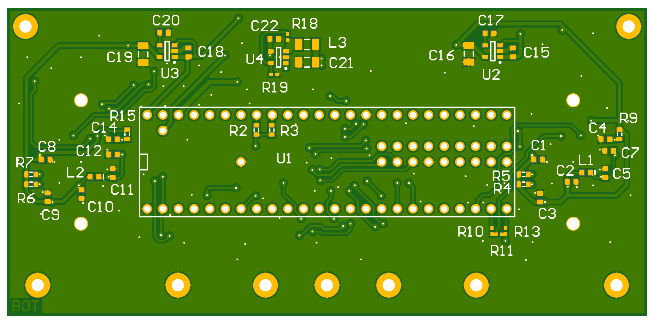
4.2.1.2. PCB design
Following some link on the Fritzing.org website, I discovered AISLER.net - german prototype PCB maker. Apparently, they are able to manufacture excellent quality 2-layer PCB for about 35 EUR, including Stencil (since then they have also added 4-layer capability). That was the reason I constrained myself to 2 layers for the TeensyCam board design. It wasn't easy to maintain signal integrity. My strategy was to route as many connections as possible on Top layer and have a more-or-less solid GND plane on Bottom layer directly below, with an effort to control high frequency return currents. Having separate voltage regulators for each sensor also helps to minimize cross-coupled noise.
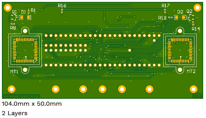
It was extremely difficult to solder the sensors to the board. I had a hard time trying to equalize solder paste deposited on pads through the stencil. Luckily, silk screen registration on the board was quite good and I used that for alignment.
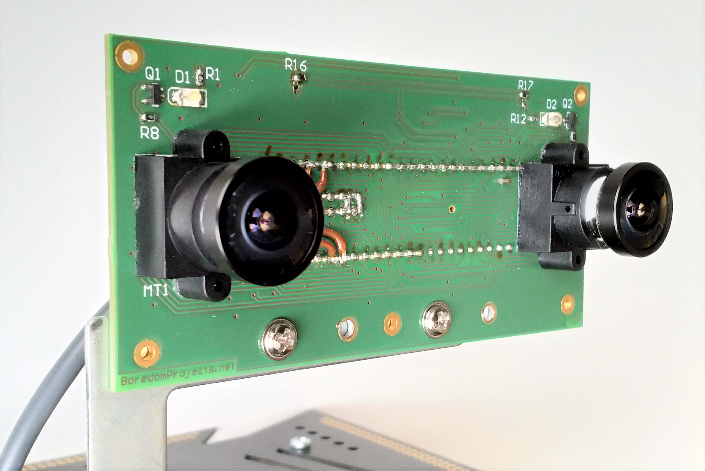
4.2.1.3. Microcontroller
I decided to use Teensy 3.6 mainly because it is quite powerful and very easy to program using Teensyduino extension to Arduino IDE. Version 3.6 in addition has a high-speed USB port capability. Besides, using a ready-made module, such as Teensy, I didn't have to bother with details of microcontroller implementation on a board.
There are two ways to read image data off of the MT9V034 sensor - parallel or serial (LVDS). The latter is not really an option, unless the sensor is interfaced to an FPGA. To read out 10-bit parallel data from sensors requires a very fast 20-lines pin reading at the rate of SYSCLK, which is 13MHz minimum. This is challenging, even for the 180MHz Teensy 3.6. The only chance to manage this would be 1) to use the sensor in Slave Mode and 2) to overclock Teensy to 240MHz, not to mention carefully monitoring generated code at the assembly-level.
Slave Mode specifically means that the exposure is controlled by providing pulses on EXPOSURE and STFRM_OUT pins simultaneously to both sensors. After that, the captured images are stored in internal buffers ready for readout at some later time by pulsing STLN_OUT pins. It took many iterations of trial-and-error experimentation before I was able to achieve correct timing.
Another trick that helped me to achieve readout timing was to group data lines from each sensor into same ports on the MK66FX1M0 chip, such that 10 bits from left sensor are connected to PTC and 10 bits from right sensor are connected to PTD. This way data lines could be sampled simultaneously within the same MOV or LDR instruction.
During debugging, I also discovered that it was helpful to capture LINE_VALID and FRAME_VALID signals together with data bus from each sensor. That is the reason I later added four wires, marked on the schematic with thick red lines.
4.2.1.4. USB interface
I initially hoped to accomplish all of the above within Arduino environment. Unfortunately, at the time of this writing, device-mode high speed USB functionality is not available for Teensy 3.6. Using the full speed mode (12Mbps) I was only able to achieve about 1 - 2 FPS rate max. I mucked about for some time and gave up.
⇒ branch teensyduino
Next, I was experimenting with uTasker, as I read good reviews about this project, specifically for its support of KINETIS line of NXP processors, including Cortex M4 of Teensy 3.6. Unfortunately, I found many things quite difficult to understand and configure. After a lot of experimentation, I was not able to achieve reliable USB CDC operation in high speed mode.
⇒ branch uTasker
While playing with uTasker, I got to know the MCUXpresso environment from NXP. This led me to the idea to try native NXP SDK and, voi la, things started to work!
⇒ branch master
The reason I decided to stick with USB CDC class instead of custom data class or perhaps Video class is that CDC is very easy to use and it is fast. I have also retained original VID/PID configuration provided by NXP SDK demo code.
The micro-USB connector on Teensy 3.6 module is only capable of full speed (12Mbps) operation. In order to establish high speed (480Mbps) USB connection, one needs to solder a separate cable to the 5-pin "USB Host Port" on the Teensy. However, in order to enable high speed device mode operation, additional hacks are needed:
- Connect external power to the VUSB input, instead of the 5V pin on the host connector
- Connect 3.3V rail to pins USB1_VBUS and VREG_IN0
Here's a diagram with highlighted connections:

4.2.2. Robotic Platform
There's been quite a few changes introduced to the platform. The main one is replacement of Raspberry Pi with a LattePanda single-board computer. This board (1st generation) is based on Intel Cherry Trail Z8350 Quad Core Processor which is significantly more powerful than Raspberry Pi 3 that I used previously. In addition, Intel architecture proved to be an advantage since the ELAS dense stereo library that I used already contains optimizations based on Intel SSE instructions.

To cope with additional power consumption mainly due to the new computer board, I had to add one more AA battery. In addition, a P-Channel MOSFET replaced one of the diodes in the battery connection circuit. This ensures very low drop-out and maximum efficiency when running on battery power. As soon as the external charger is inserted, the MOSFET shuts off and disconnects battery from load. The power is then routed to the system through the diode.
I noticed that it is absolutely essential to provide rock steady supply voltage to the LattePanda in order to prevent sporadic restarts. To this end I added one more 5V switch-mode regulator (MP1584EN) to power auxiliary circuitry. This way the main 5V switcher - S18V20F5 - is dedicated to LattePanda and is able to deliver to it up to 3A of peak current.
Communication with slave microcontroller (Teensy 3.2) is now running over USB using CDC profile. This was easy to implement using existing MessageSerial module. A proportional-on-measurement control mode was added to the motor PID controllers together with the automatic motor shutdown functionality if no commands received for some time.
Slave microcontroller firmware is here: https://github.com/icboredman/cherokey_slave.git
Complete Platform Schematics:

Another major addition to this robot is the ability to speak and understand speech! Well, sort of :) That's why there is a microphone and an amplifier with speaker on the schematic diagram. Software components to enable this functionality are explained in next sections.
I used a small condenser usb microphone and a 2W, 8 ohm speaker, 28 mm in diameter. Speaker is driven by a nice little class-D amplifier module - Adafruit PAM8302A - with volume control.
 |
|
 |

Finally, I noticed that during peaks of activity, the processor can get very hot, sometimes to the point of throttling. Obviously, little heat sinks glued to the metal lid were not adequate to properly cool the device. So, I added a small fan. And what is a better way to control the fan if not with the Arduino MCU embedded within LattePanda board itself? The idea was to spin the fan only when needed and as fast as needed to keep overall power efficiency.
The sketch for the embedded Leonardo is pretty simple. It receives a one byte temperature over serial connection and uses it to control the cooling fan through PWM on pin 9. LED blinking rate serves as a visual indicator of current temperature.
Arduino Leonardo sketch: fan_controller.ino
Since I didn't have a suitable switch to drive the fan handy, I used a logic level shifter board for this purpose. It turned out very convenient to attach to the LattePanda using a few header sockets.

4.3. Software
All source code on GitHub:
| nav_controller_node | ROS node that controls robot by sending goals to Navigation Stack | |
| camera_node | ROS node that manages interface to stereo camera module | |
| base_serial_node | ROS node that enables communication with robot base over a serial link | |
| cherokey_ws | ROS workspace that ties it all together |
4.3.1. Localization and Navigation
A major drawback of stereo camera as a range measuring device vs. laser scanner is that the accuracy of measurement degrades very quickly with distance. This is obviously the result of angular measurements that disparity calculations are based on. Practically this means that contours of detected objects can only be used reliably in close proximity, such as during collision avoidance. Shapes of objects farther from camera, on the other hand, appear too noisy and wobbly (see error analysis). That is the reason my first attempt of localization failed, since I used emulated laser scan generated from camera depth map as an input to AMCL (part of ROS navigation stack). AMCL was not able to reliably match noisy emulated laser scans with previously recorder contours.
The solution came after I realized that camera provides much more information than a simple 2D laser scan. It gives a whole image of the scene. If this appearance information could be recorded and later retrieved and matched, the problem of localization would be solved. Turns out, there is a large computer vision research area covering exactly that. Among many existing appearance-based SLAM approaches, I settled on RTAB-Map tool kit, which is open-source, ROS-ready and claims to be real-time, i.e. suitable for embedded (low resource) computing platforms.
At a very simplistic level, appearance-based SLAM works like this:
Stereo camera delivers image+depth representation of a scene, which is stored in a database along with the scene's relative position and orientation derived from odometry. As robot moves in the environment, new scenes are added to the database together with their position. At each step, however, a matching process takes place that tries to compare new scene with all previously remembered ones. When a match is found, robot's position and orientation offset is computed relative to the matched scene. This offset is used to adjust current location and to correct odometry errors of a sequence of previously recorded locations in a process called loop closure. As a result, an accurate map of the environment is being created.
We, humans use exactly the same "algorithm" to orient ourselves in our environment. When we, for example, emerge from a subway station to a city street, first thing we do is to look around trying to find a familiar landmark. As soon as we recognize a scene, we immediately understand where we are and which way we have to go. I find it very cool! :-)
The following video illustrates appearance-based localization and loop closure detection. Whenever RTAB-Map successfully finds a match, it outputs a 3D point cloud of the scene and returns corrected pose+covariance in the form of tf transform map→odom.
In the above video, robot contour is initially placed at the uncorrected pose which is adjusted whenever loop closure is detected. Green arrow indicates current goal and red arrow is the corrected pose with covariance.
Here's a video of Kidnapped Robot Test:
After the hand-of-god finally delivers robot to new location, it takes a few seconds before Heisenberg successfully re-orients himself!
rtabmap-ros package can be used in two modes: mapping and localization. After a one-time mapping session, the generated database is reused in localization mode which delivers a static map of the environment (created as a projection of 3D point-cloud scenes on a 2D surface) to a navigation/planner node.
At the ROS level, the nodes are connected similar to this rtabmap tutorial which also uses a fake laser scan generated from camera depth images.

The camera node generates depth map and together with image from left camera passes it to a little nodelet rgbd_sync that performs synchronization and converts this information into the rtabmap's native format - rgbd_image topic. rtabmap also received odom transform from the base controller and runs localization process.
move_base receives global map from rtabmap in the form of 2D projected occupancy grid as well as the tf transform map→odom. The emulated laser scan is used only within move_base for updating local occupancy grid, i.e. for collision avoidance.
The whole process is orchestrated by nav_controller node that receives spoken or typed commands and registers navigation goals using actionlib protocol.
The main launch file that references all other configuration and actually brings-up the robot in navigation mode is here: nav_controller.launch
4.3.1.1. Installation
Unfortunately, pre-built binaries of RTAB-Map for current ROS distributions do not include some nice features like SIFT or SURF. To get them working, it is necessary to install rtabmap_ros from source, as described here, and before that, to install OpenCV from source while enabling non-free modules, like this.
4.3.2. Mapping
There are basically three ways to run SLAM algorithm using RTAB-Map tool kit. The choice depends on application needs and the available computing power:
- Online
- everything done within robot itself
- high load requirement on embedded computer
- Remote
- RTAB-Map runs on remotely connected computer
- mapping is achieved in real-time
- computing power partially offloaded to remote processor
- high network bandwidth, low latency requirements
- Offline
- sensor and odometry messages are recorded in a ROS bag
- RTAB-Map runs on remote computer at a later time
- map is generated not in real time
In all these cases, the robot is being manually driven around using teleop_key_node. I have not considered fully autonomous exploratory mapping+navigation yet.
Only the last case - offline mapping - has so far provided good results. My plan is to continue working on case 2 in the future.
4.3.2.1. Online, real-time
I found that Online mapping was definitely too much for the LattePanda. Besides, considering that in my application the map had to be created only once, there was no real need to run SLAM in real-time. However, here's an example of setup that I've been playing with:
on robot:roslaunch nav_rtabmap rtab_slam.launchrosrun teleop_key teleop_key_node
on remote, at the same time:roslaunch rtabmapviz_remote.launch or rviz -d ~/.rviz/nav_rtab.rviz
The launch file is here: rtab_slam.launch and /remote/rtabmapviz_remote.launch
4.3.2.2. Remote, real-time
The idea here is to offload main SLAM computing requirements to the remote processor. The robot only collects and transmits real-time sensor/odometry info over the network to the remote running RTAB-Map. The critical element in this case is the network bandwidth and latency. It becomes important to find a right amount of compression applied to sensor messages to achieve a good balance between processor loading and network latency. One example of how RTAB-Map proposes to do that is here: rtabmap_ros remote mapping tutorial.
on robot:roslaunch nav_rtabmap rtab_slam_remote.launchrosrun teleop_key teleop_key_node cmd_vel:=/robot/cmd_vel
on remote, at the same time:roslaunch remote_slam.launch ← this will also launch rtabmapviz node
It helps to run the synchronizing nodelet rgbd_sync on the robot, such that all topics from camera are collected together, synchronized and compressed into rgbd_image topic before being sent over network.
This seems to me the best approach to mapping for this type of robot. The real-time aspect is quite useful for immediate feedback from mapping to tele-op-ing, for example, to revisit key scenes important for loop closure detection.
Launch files: rtab_slam_remote.launch and /remote/remote_slam.launch
4.3.2.3. Offline, separate sessions
Here, the idea is to use ROS bag recording capability to store all sensor information, odometry, tf, etc. while manually driving robot around. Later, this bag is transferred to the remote computer, played back and fed to RTAB-Map running in mapping mode.
on robot:roslaunch nav_rtabmap rtab_slam_remote.launchrosbag record /robot/rgbd_image /robot/battery /robot/odom /tfrosrun teleop_key teleop_key_node cmd_vel:=/robot/cmd_vel
on remote, at a later session:rosbag play --clock the-big-fat-bag-file.bagrosparam set use_sim_time "true"roslaunch remote_slam.launch ← this will also launch rtabmapviz node
The advantage of this approach is relaxed requirements on robot computing power as well as on its network bandwidth.
The disadvantage is the lack of real-time feedback between mapping results and manual tele-operation. The key scenes used for loop closure have to be guessed in advance during bag recording with hope that enough of these key places have been revisited to make a good map. It took me a few trials to achieve a good data set for the mapping session.
4.3.3. Speech
4.3.3.1. Listening
Voice recognition has not been the primary goal of this project. Once I got navigation to work, I was looking for an easy way to give commands to the robot. Setting up goals by pointing and clicking in RViz was not very convenient. Since I am, as far as I know, human, spoken words seem to be the most natural way for me to give my commands to the robot. So I decided to try to teach Heisenberg to recognize speech.
Among many existing ways to analyze and process speech, CMUSphinx tool kit appears to be the most popular in the category of offline speech-to-text tools suitable for resource-limited, embedded applications. Besides, this library is open source, well documented and easy to use.
I followed this great post to install and configure PocketSphinx component. I could not get good results with analog input (3.5 mm jack) on the LattePanda board, so I purchased a nice small USB microphone. I also adapted standard us-english acoustic model as described here to better match my particular pronunciation and microphone characteristics.
The basic strategy of my speech recognition process is a keyword spotting mode followed by a grammar-based command recognition, all implemented within the nav_controller_node.
One of the reason I named my robot "Heisenberg" was that this is a nice long quite unique sounding phrase, resulting in a reliable keyword spotting response. The keyword file is here: nav_controller_node/sphinx/keyphrase.list and the grammar rules file in JSGF format is: nav_controller_node/sphinx/grammar.jsgf.
Once nav_controller_node recognizes a command, the keyword from JSGF file is matched with commands in the nav_controller_node/goals.yaml file, for example GO, MOVE, TURN, etc. Some of these commands may have a parameter associated with it, such as GO command is then matched with destination word, for example HOME, KITCHEN. Finally, these destinations also contain a set of coordinates in a form of quaternions which may be absolute or relative (some components are zeros).
The reason all words in the above files are capitalized is that I used this online language model tool to build dictionary that would include new words like "Heisenberg".
4.3.3.2. Talking
After Heisenberg learned to understand spoken commands, teaching it to speak was quite simple. The library of choice here is eSpeak-NG, since it is open-source, easy to use, very popular and well documented. Although the generated speech still sounds a bit robot-like, in my case this was an advantage. The most natural sounding speech is produced using MBROLA synthesizer component and its voices data set.
Here's an example of Heisenberg speaking:
He still needs to work on the speech intonation, but I kinda like his a bit grumpy personality. :-)
4.3.4. Cooling Fan
At some point it became apparent that during peaks of activity processor would start throttling by lowering its performance. That's when I decided to implement active temperature control using a fan.
There is a neat little way to get a reading of current processor temperature from Linux, which is described in this forum post.
Reading the temperature on LattePanda results in the following:
cat /sys/class/thermal/thermal_zone*/type
acpitz
INT3400 Thermal
STR0
PNIT
soc_dts0
soc_dts1
and
cat /sys/class/thermal/thermal_zone*/temp
0
20000
-273200
61000
51000
37000
It is actually the fourth item that seems to contain main CPU temperature: PNIT = 61°C.
What remained was to code this into base_serial_node and send the temperature to Arduino Leonardo embedded within LattePanda board. It, in turn, would control spin rate of the fan using PWM and keep the temperature down. Arduino sketch: fan_controller.ino.
CPU throttling can be monitored by comparing nominal CPU frequency:
cat /sys/devices/system/cpu/cpu0/cpufreq/cpuinfo_max_freq
against actual frequency under load:
sudo cat /sys/devices/system/cpu/cpu3/cpufreq/cpuinfo_cur_freq
In my case cpuinfo_cur_freq starts to go down when the core temperature approaches 80°C. With the implemented active fan control, the temperature goes only up to about 65°C under heavy load.